

The following discusses the use of computerized active room optimization and as an example a technology which was developed by “Harman” called Sound Field Management or SFM.
Figure 1: Example of a multiple loudspeaker and multiple listener scenario.
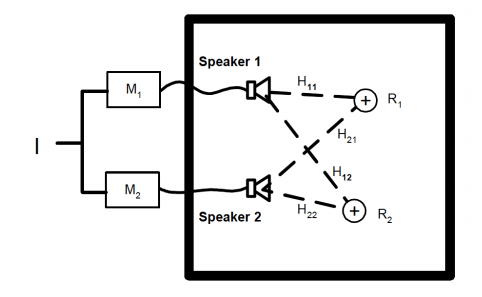
I is the signal input, delivered to multiple loudspeakers. M1, M2 are the modification factors and R1, R2 represent the two different frequency responses at the listening locations. H11 through H22 are the transfer functions between the loudspeakers and each listener.
Equations and Calculations!
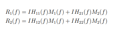
The optimization scenario can be considered to be a time invariant and linear system and can be given in the frequency domain in equation 1. as:
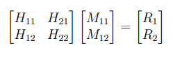
The input I can is assumed to be unity and the set of linear equations can be written in matrix form as:
The optimization reaches the optimum in case of an equal frequency response at each listening location and will occur for R equal unity.
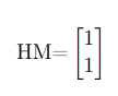
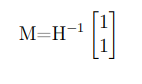
A proper inverse of H has to be found and 3.9 can be reduced to equation 5:
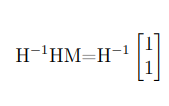
This eventually leads to the required modifier M and only has to be calculated for frequencies that require optimization.
In this post, we explained first part of Subwoofer Placement Combined with Signal Processing; Other types of these methods that need to be mentioned to improve the sound will be published in future posts. These will pave the way for creating a home theater of the highest quality.
Although, we explored two types of sound absorbers that are effective in controlling sound reflections; Other types of these absorbers and the things that need to be mentioned to improve the sound will be published in future posts. These will pave the way for creating a home theater of the highest quality.

